Figure 21.2 Packet exchange and RTT measurement.
TCP provides a reliable transport layer. One of the ways it provides reliability is for each end to acknowledge the data it receives from. the other end. But data segments and acknowledgments can get lost. TCP handles this by setting a timeout when it sends data, and if the data isn't acknowledged when the timeout expires, it retransmits the data. A critical element of any implementation is the timeout and retransmission strategy. How is the timeout interval determined, and how frequently does a retransmission occur?
We've already seen two examples of timeout and retransmission: (1) In the ICMP port unreachable example in Section 6.5 we saw the TFTP client using UDP employing a simple (and poor) timeout and retransmission strategy: it assumed 5 seconds was an adequate timeout period and retransmitted every 5 seconds. (2) In the ARP example to a nonexistent host (Section 4.5), we saw that when TCP tried to establish the connection it retransmitted its SYN using a longer delay between each retransmission. TCP manages four different timers for each connection.
In this chapter we start with a simple example of
TCP's timeout and retransmission and then move to a larger example
that lets us look at all the details involved in TCP's timer management.
We look at how typical implementations measure the round-trip
time of TCP segments and how TCP uses these measurements to estimate
the retransmission timeout of the next segment it transmits. We
then look at TCP's congestion avoidance-what TCP does when packets
are lost-and follow through an actual example where packets are
lost. We also look at the newer fast retransmit and fast recovery
algorithms, and see how they let TCP detect lost packets faster
than waiting for a timer to expire.
21.2 Simple Timeout and Retransmission Example
Let's first look at the retransmission strategy used by TCP. We'll establish a connection, send some data to verify that everything is OK, disconnect the cable, send some more data, and watch what TCP does:
| bsdi % telnet svr4 discard | |
| Trying 140.252.13.34... | |
| Connected to svr4. | |
| Escape character is '^]'. | |
| Hello, world | send this line normally |
| and hi | disconnect cable before sending this line |
| Connection closed by foreign host. | output whenTCP gives up after 9 minutes |
Figure 21.1 shows the tcpdump output. (We have removed all the type-of-service information that is set by bsdi.)
| 1 | 0.0 | bsdi.1029 > svr4.discard: S 1747921409:1747921409(0)
win 4096 <mss 1024> |
| 2 | 0.004811 ( 0.0048) | svr4.discard > bsdi.1029: S 3416685569:3416685569(0)
ack 1747921410 win 4096 <mss 1024> |
| 3 | 0.006441 ( 0.0016) | bsdi.1029 > svr4.discard: . ack 1 win 4096 |
| 4 | 6.102290 ( 6.0958) | bsdi.1029 > svr4.discard: P 1:15(14) ack 1 win 4096 |
| 5 | 6.259410 ( 0.1571) | svr4.discard > bsdi.1029: . ack 15 win 4096 |
| 6 | 24.480158 (18.2207) | bsdi.1029 > svr4.discard: P 15:23(8) ack 1 win 4096 |
| 7 | 25.493733 ( 1.0136) | bsdi.1029 > svr4.discard: P 15:23(8) ack 1 win 4096 |
| 8 | 28.493795 ( 3.0001) | bsdi.1029 > svr4.discard: P 15:23(8) ack 1 win 4096 |
| 9 | 34.493971 ( 6.0002) | bsdi.1029 > svr4.discard: P 15:23(8) ack 1 win 4096 |
| 10 | 46.484427 (11.9905) | bsdi.1029 > svr4.discard: P 15:23(8) ack 1 win 4096 |
| 11 | 70.485105 (24.0007) | bsdi.1029 > svr4.discard: P 15:23(8) ack 1 win 4096 |
| 12 | 118.486408 (48.0013) | bsdi.1029 > svr4.discard: P 15:23(8) ack 1 win 4096 |
| 13 | 182.488164 (64.0018) | bsdi.1029 > svr4.discard: P 15:23(8) ack 1 win 4096 |
| 14 | 246.489921 (64.0018) | bsdi.1029 > svr4.discard: P 15:23(8) ack 1 win 4096 |
| 15 | 310.491678 (64.0018) | bsdi.1029 > svr4.discard: P 15:23(8) ack 1 win 4096 |
| 16 | 374.493431 (64.0018) | bsdi.1029 > svr4.discard: P 15:23(8) ack 1 win 4096 |
| 17 | 438.495196 (64.0018) | bsdi.1029 > svr4.discard: P 15:23(8) ack 1 win 4096 |
| 18 | 502.486941 (63.9917) | bsdi.1029 > svr4.discard: P 15:23(8) ack 1 win 4096 |
| 19 | 566.488478 (64.0015) | bsdi.1029 > svr4.discard: R 23:23(0) ack 1 win 4096 |
Lines 1, 2, and 3 correspond to the normal TCP connection establishment. Line 4 is the transmission of "hello, world" (12 characters plus the carriage return and linefeed), and line 5 is its acknowledgment. We then disconnect the Ethernet cable from svr4.
Line 6 shows "and hi" being sent. Lines 7-18 are 12 retransmissions of that segment, and line 19 is when the sending TCP finally gives up and sends a reset.
Examine the time difference between successive retransmissions: with rounding they occur 1, 3, 6, 12, 24, 48, and then 64 seconds apart. We'll see later in this chapter that the first timeout is actually set for 1.5 seconds after the first transmission. (The reason it occurs 1.0136 seconds after the first transmission, and not exactly 1.5 seconds, was explained in Figure 18.7.) After this the timeout value is doubled for each retransmission, with an upper limit of 64 seconds.
This doubling is called an exponential backoff. Compare this to the TFTP example in Section 6.5, where every retransmission occurred 5 seconds after the previous.
The time difference between the first transmission of the packet (line 6 at time 24.480) and the reset (line 19 at time 566.488) is about 9 minutes. Modem TCP's are persistent when trying to send data!
On most implementations this total timeout value
is not tunable. Solaris 2.2 allows the administrator to change
this (the tcp_ip_abort_interval variable in Section E.4) and its
default is only 2 minutes, not the more common 9 minutes.
21.3 Round-Trip Time Measurement
Fundamental to TCP's timeout and retransmission is the measurement of the round-trip time (RTT) experienced on a given connection. We expect this can change over time, as routes might change and as network traffic changes, and TCP should track these changes and modify its timeout accordingly.
First TCP must measure the RTT between sending a byte with a particular sequence number and receiving an acknowledgment that covers that sequence number. Recall from the previous chapter that normally there is not a one-to-one correspondence between data segments and ACKs. In Figure 20.1 this means that one RTT that can be measured by the sender is the time between the transmission of segment 4 (data bytes 1-1024) and the reception of segment 7 (the ACK of bytes 1-2048), even though this ACK is for an additional 1024 bytes. We'll use M to denote the measured RTT.
The original TCP specification had TCP update a smoothed RTT estimator (called R) using the low-pass filter
where a is a smoothing factor with a recommended value of 0.9. This smoothed RTT is updated every time a new measurement is made. Ninety percent of each new estimate is from the previous estimate and 10% is from the new measurement.
Given this smoothed estimator, which changes as the RTT changes, RFC 793 recommended the retransmission timeout value (RTO) be set to
where b is a delay variance factor with a recommended value of 2.
[Jacobson 1988] details the problems with this approach, basically that it can't keep up with wide fluctuations in the RTT, causing unnecessary retransmissions. As Jacobson notes, unnecessary retransmissions add to the network load, when the network is already loaded. It is the network equivalent of pouring gasoline on a fire.
What's needed is to keep track of the variance in the RTT measurements, in addition to the smoothed RTT estimator. Calculating the RTO based on both the mean and variance provides much better response to wide fluctuations in the round-trip times, than just calculating the RTO as a constant multiple of the mean. Figures 5 and 6 in [Jacobson 1988] show a comparison of the RFC 793 RTO values for some actual round-trip times, versus the RTO calculations we show below, which take into account the variance of the round-trip times.
As described by Jacobson, the mean deviation is a good approximation to the standard deviation, but easier to compute. (Calculating the standard deviation requires a square root.) This leads to the following equations that are applied to each RTT measurement M.
where A is the smoothed RTT (an estimator of the average) and D is the smoothed mean deviation. Err is the difference between the measured value just obtained and the current RTT estimator. Both A and D are used to calculate the next retransmission timeout (RTO). The gain g is for the average and is set to 1/8 (0.125). The gain for the deviation is h and is set to 0.25. The larger gain for the deviation makes the RTO go up faster when the RTT changes.
[Jacobson 1988] specified 2D in the calculation of
RTO, but after further research, [Jacobson 1990c] changed the
value to 4D, which is what appeared in the BSD Net/1 implementation.
Jacobson specifies a way to do all these calculations
using integer arithmetic, and this is the implementation typically
used. (That's one reason g, h, and the multiplier 4 are
all powers of 2, so the operations can be done using shifts instead
of multiplies and divides.)
Comparing the original method with Jacobson's, we
see that the calculations of the smoothed average are similar
(a is one minus the gain g) but a different gain
is used. Also, Jacobson's calculation of the RTO depends
on both the smoothed RTT and the smoothed mean deviation, whereas
the original method used a multiple of the smoothed RTT.
We'll see how these estimators are initialized in
the next section, when we go through an example.
A problem occurs when a packet is retransmitted.
Say a packet is transmitted, a timeout occurs, the RTO
is backed off as shown in Section 21.2, the packet is retransmitted
with the longer RTO, and an acknowledgment is received.
Is the ACK for the first transmission or the second? This is called
the retransmission ambiguity problem.
[Karn and Partridge 1987] specify that when a timeout
and retransmission occur, we cannot update the RTT estimators
when the acknowledgment for the retransmitted data finally arrives.
This is because we don't know to which transmission the ACK corresponds.
(Perhaps the first transmission was delayed and not thrown away,
or perhaps the ACK of the first transmission was delayed.)
Also, since the data was retransmitted, and the exponential
backoff has been applied to the RTO, we reuse this backed off
RTO for the next transmission. Don't calculate a new RTO until
an acknowledgment is received for a segment that was not retransmitted.
We'll use the following example throughout this chapter
to examine various implementation details of TCP's timeout and
retransmission, slow start, and congestion avoidance.
Using our sock program,
32768 bytes of data are sent from our host slip
to the discard service on the host vangogh.cs.berkeley.edu
using the command:
slip % sock -D -i -n32
vangogh.cs.berkeley.edu discard
From the figure on the inside front cover, slip
is connected from the 140.252.1 Ethernet by two SLIP links, and
from there across the Internet to the destination. With two 9600
bits/sec SLIP links, we expect some measurable delays.
This command performs 32 1024-byte writes, and since
the MTU between slip and bsdi
is 296, this becomes 128 segments, each with 256 bytes of user
data. The total time for the transfer is about 45 seconds and
we see one timeout and three retransmissions.
While this transfer was running we ran tcpdump
on the host slip and captured all
the segments sent and received. Additionally we specified the
-D option to turn on socket debugging
(Section A.6). We were then able to run a modified version of
the trpt(8) program to print numerous
variables in the connection control block relating to the round-trip
timing, slow start, and congestion avoidance.
Given the volume of trace output, we can't show it
all. Instead we'll look at pieces as we proceed through the chapter.
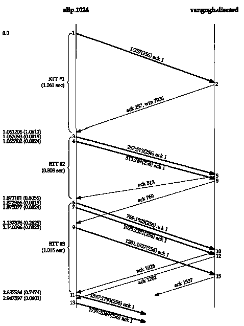
Figure 21.2 shows the transfer of data and acknowledgments for
the first 5 seconds. We have modified this output slightly from
our previous display of tcpdump output.
Although we only measure the times that the packet is sent or
received on the host running tcpdump,
in this figure we want to show that the packets are crossing in
the network (which they are, since this LAN connection is not
like a shared Ethernet), and show when the receiving host is probably
generating the ACKs. (We have also removed all the window advertisements
from this figure, slip always advertised
a window of 4096, and vangogh always
advertised a window of 8192.)
Karn's Algorithm
21.4 An RTT Example
Also note in this figure that we have numbered the segments 1-13 and 15, in the order in which they were sent or received on the host slip. This correlates with the tcpdump output that was collected on this host.
Three curly braces have been placed on the left side of the time line indicating which segments were timed for RTT calculations. Not all data segments are timed.
Most Berkeley-derived implementations of TCP measure only one RTT value per connection at any time. If the timer for a given connection is already in use when a data segment is transmitted, that segment is not timed.
The timing is done by incrementing a counter every time the 500-ms TCP timer routine is invoked. This means that a segment whose acknowledgment arrives 550 rns after the segment was sent could end up with either a 1 tick RTT (implying 500 ms) or a 2 tick RTT (implying 1000 ms).
In addition to this tick counter for each connection, the starting sequence number of the data in the segment is also remembered. When an acknowledgment that includes this sequence number is received, the timer is turned off. If the data was not retransmitted when the ACK arrives, the smoothed RTT and smoothed mean deviation are updated based on this new measurement.
The timer for the connection in Figure 21.2 is started when segment 1 is transmitted, and turned off when its acknowledgment (segment 2) arrives. Although its RTT is 1.061 seconds (from the tcpdump output), examining the socket debug information shows that three of TCP's clock ticks occurred during this period, implying an RTT of 1500 ms.
The next segment timed is number 3. When segment 4 is transmitted 2.4 ms later, it cannot be timed, since the timer for this connection is already in use. When segment 5 arrives, acknowledging the data that was being timed, its RTT is calculated to be 1 tick (500 ms), even though we see that its RTT is 0.808 seconds from the tcpdump output.
The timer is started again when segment 6 is transmitted, and turned off when its acknowledgment (segment 10) is received 1.015 seconds later. The measured RTT is 2 clock ticks. Segments 7 and 9 cannot be timed, since the timer is already being used. Also, when segment 8 is received (the ACK of 769), nothing is updated since the acknowledgment was not for bytes being timed.
Figure 21.3 shows the relationship in this example between the actual RTTs that we can determine from the tcpdump output, and the counted clock ticks.
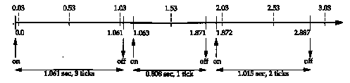
On the top we show the clock ticks, every 500 ms. On the bottom we show the times output by tcpdump, and when the timer for the connection is turned on and off. We know that 3 ticks occur between sending segment 1 and receiving segment 2, 1.061 seconds later, so we assume the first tick occurs at time 0.03. (The first tick must be between 0.00 and 0.061.) The figure then shows how the second measured RTT was counted as 1 tick, and the third as 2 ticks.
In this complete example, 128 segments were transmitted, and 18 RTT samples were collected. Figure 21.4 shows the measured RTT (taken from the tcpdump output) along with the RTO used by TCP for the timeout (taken from the socket debug output). The x-axis starts at time 0 in Figure 21.2, when the first data segment is transmitted, not when the first SYN is transmitted.
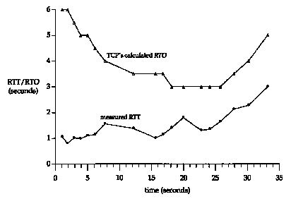
The first three data points for the measured RTT correspond to the 3 RTTs that we show in Figure 21.2. The gaps in the RTT samples around times 10, 14, and 21 are caused by retransmissions that took place there (which we'll show later in this chapter). Kam's algorithm prevents us from updating our estimators until another segment is transmitted and acknowledged. Also note that for this implementation, TCP's calculated RTO is always a multiple of 500 ms.
Let's see how the RTT estimators (the smoothed RTT and the smoothed mean deviation) are initialized and updated, and how each retransmission timeout is calculated.
The variables A and D are initialized to 0 and 3 seconds, respectively. The initial retransmission timeout is calculated using the formula
(The factor 2D is used only for this initial
calculation. After this 4D is added to A to calculate RTO,
as shown earlier.) This is the RTO for the transmission
of the initial SYN.
It turns out that this initial SYN is lost, and we
time out and retransmit. Figure 21.5 shows the first four lines
from the tcpdump
output file.
When the timeout occurs after 5.802 seconds, the
current RTO is calculated as
The exponential backoff is then applied to the RTO
of 12. Since this is the first timeout we use a multiplier of
2, giving the next timeout value as 24 seconds. The next timeout
is calculated using a multiplier of 4, giving a value of 48 seconds:
12 x 4. (These initial RTOs for the first SYN on a connection,
6 seconds and then 24 seconds, are what we saw in Figure 4.5.)
The ACK arrives 467 ms after the retransmission.
The values of A and D are not updated, because of Karn's
algorithm dealing with the retransmission ambiguity. The next
segment sent is the ACK on line 4, but it is not timed since it
is only an ACK. (Only segments containing data are timed.)
When the first data segment is sent (segment 1 in
Figure 21.2) the RTO is not changed, again owing to Karn's algorithm.
The current value of 24 seconds is reused until an RTT measurement
is made. This means the RTO for time 0 in Figure 21.4 is really
24, but we didn't plot that point.
When the ACK for the first data segment arrives (segment
2 in Figure 21.2), three clock ticks were counted and our estimators
are initialized as
(The value 1.5 for M is for 3 clock ticks.)
The previous initialization of A and D to 0 and
3 was for the initial RTO calculation. This initialization is
for the first calculation of the estimators using the first RTT
measurement M. The RTO is calculated as
When the ACK for the second data segment arrives
(segment 5 in Figure 21.2), 1 clock tick is counted (0.5 seconds)
and our estimators are updated as
There are some subtleties in the fixed-point representations
of Err, A, and D, and the fixed-point calculations
that are actually used (which we've shown in floating-point for
simplicity). These differences yield an RTO of 6 seconds
(not 6.3125), which is what we plot in Figure 21.4 for time 1.871.
We described the slow start algorithm in Section 20.6.
We can see it in action again in Figure 21.2.
Only one segment is initially transmitted on the
connection, and its acknowledgment must be received before another
segment is transmitted. When segment 2 is received, two more segments
are transmitted.
Now let's look at the transmission of the data segments.
Figure 21.6 is a plot of the starting sequence number in a segment
versus the time that the segment was sent. This provides a nice
way to visualize the data transmission. Normally the data points
should move up and to the right, with the slope of the points
being the transfer rate. Retransmissions will appear as motion
down and to the right.
At the beginning of Section 21.4 we said the total
time for the transfer was about 45 seconds, but we show only 35
seconds in this figure. These 35 seconds account for sending the
data segments only. The first data segment was not transmitted
until 6.3 seconds after the first SYN was sent, because the first
SYN appears to have been lost and was retransmitted (Figure 21.5).
Also, after the final data segment and the FIN were sent (at time
34.1 in Figure 21.6) it took another 4.0 seconds to receive the
final 14 ACKs from the receiver, before the receiver's FIN was
received.
We can immediately see the three retransmissions
around times 10, 14, and 21 in Figure 21.6. At each of these three
points we can also see that only one segment is retransmitted,
because only one dot dips below the upward slope.
Let's examine the first of these dips in detail (around
the 10-second mark). From the tcpdump
output we can put together Figure 21.7.
We have removed all the window advertisements from
this figure, except for segment 72, which we discuss below, slip
always advertised a window of 4096, and vangogh
advertised a window of 8192. The segments are numbered in this
figure as a continuation of Figure 21.2, where the first data
segment across the connection was numbered 1. As in Figure 21.2,
the segments are numbered according to their send or receive order
on the host slip, where tcpdump
was being run. We have also removed a few segments that have no
relevance to the discussion (44, 47, and 49, all ACKs from vangogh).
It appears that segment 45 got lost or arrived damaged-we
can't tell from this output. What we see on the host slip
is the acknowledgment for everything up through but not including
byte 6657 (segment 58), followed by eight more ACKs of this same
sequence number. It is the reception of segment 62, the third
of the duplicate ACKs, that forces the retransmission of the data
starting at sequence number 6657 (segment 63). Indeed, Berkeley-derived
implementations count the number of duplicate ACKs received, and
when the third one is received, assume that a segment has been
lost and retransmit only one segment, starting with that sequence
number. This is Jacobson's fast retransmit algorithm, which
is followed by his fast recovery algorithm. We discuss
both algorithms in Section 21.7.
Notice that after the retransmission (segment 63),
the sender continues normal data transmission (segments 67, 69,
and 71). TCP does not wait for the other end to acknowledge the
retransmission.
Let's examine what happens at the receiver. When
normal data is received in sequence (segment 43), the receiving
TCP passes the 256 bytes of data to the user process. But the
next segment received (segment 46) is out of order: the starting
sequence number of the data (6913) is not the next expected sequence
number (6657). TCP saves the 256 bytes of data and responds with
an ACK of the highest sequence number successfully received, plus
one (6657). The next seven segments received by vangogh
(48, 50, 52, 54, 55, 57, and 59) are also out of order. The data
is saved by the receiving TCP, and duplicate ACKs are generated.
Currently there is no way for TCP to tell the other
end that a segment is missing. Also, TCP cannot acknowledge out-of-order
data. All vangogh can do at this
point is continue sending the ACKs of 6657.
When the missing data arrives (segment 63), the receiving
TCP now has data bytes 6657-8960 in its buffer, and passes these
2304 bytes to the user process. All 2304 bytes are acknowledged
in segment 72. Also notice that this ACK advertises a window of
5888 (8192 - 2304), since the user process hasn't had a chance
to read the 2304 bytes that are ready for it.
If we look in detail at the tcpdump
output for the dips around times 14 and 21 in Figure 21.6, we
see that they too were caused by the receipt of three duplicate
ACKs, indicating that a packet had been lost. In each of these
cases only a single packet was retransmitted.
We'll continue this example in Section 21.8, after
describing more about the congestion avoidance algorithms.
Slow start, which we described in Section 20.6, is
the way to initiate data flow across a connection. But at some
point we'll reach the limit of an intervening router, and packets
can be dropped. Congestion avoidance is a way to deal with lost
packets. It is described in [Jacobson 1988].
The assumption of the algorithm is that packet loss
caused by damage is very small (much less than 1%), therefore
the loss of a packet signals congestion somewhere in the network
between the source and destination. There are two indications
of packet loss: a timeout occurring and the receipt of duplicate
ACKs. (We saw the latter in Section 21.5. If we are using a timeout
as an indication of congestion, we can see the need for a good
RTT algorithm, such as that described in Section 21.3.)
Congestion avoidance and slow start are independent
algorithms with different objectives. But when congestion occurs
we want to slow down the transmission rate of packets into the
network, and then invoke slow start to get things going again.
In practice they are implemented together.
Congestion avoidance and slow start require that
two variables be maintained for each connection: a congestion
window, cwnd, and a slow start threshold size, ssthresh.
The combined algorithm operates as follows:
Congestion avoidance is flow control imposed by the
sender, while the advertised window is flow control imposed by
the receiver. The former is based on the sender's assessment of
perceived network congestion; the latter is related to the amount
of available buffer space at the receiver for this connection.
If cwnd is less than or equal to ssthresh,
we're doing slow start; otherwise we're doing congestion avoidance.
Slow start continues until we're halfway to where we were when
congestion occurred (since we recorded half of the window size
that got us into trouble in step 2), and then congestion avoidance
takes over.
Slow start has cwnd start at one segment,
and be incremented by one segment every time an ACK is received.
As mentioned in Section 20.6, this opens the window exponentially:
send one segment, then two, then four, and so on.
Congestion avoidance dictates that cwnd be
incremented by 1/cwnd each time an ACK is received. This
is an additive increase, compared to slow start's exponential
increase. We want to increase cwnd by at most one segment
each round-trip time (regardless how many ACKs are received in
that RTT), whereas slow start will increment cwnd by the
number of ACKs received in a round-trip time.
All 4.3BSD releases and 4.4BSD incorrectly add a
small fraction of the segment size (the segment size divided by
8) during congestion avoidance. This is wrong and should not be
emulated in future releases [Floyd 1994]. Nevertheless, we show
this term in future calculations, to arrive at the same answer
as the (incorrect) implementation.
The 4.3BSD Tahoe release, described in [Leffler et
al. 1989], performed slow start only if the other end was on a
different network. This was changed with the 4.3BSD Reno release
so that slow start is always performed.
Figure 21.8 is a visual description of slow start
and congestion avoidance. We show cwnd and ssthresh
in units of segments, but they're really maintained in bytes.
In this figure we assume that congestion occurred
when cwnd had a value of 32 segments. ssthresh is
then set to 16 segments and cwnd is set to 1 segment. One
segment is then sent at time 0 and assuming its ACK is returned
at time 1, cwnd is incremented to 2 segments. Two segments
are then sent and assuming their ACKs return by time 2, cwnd
is incremented to 4 segments (once for each ACK). This exponential
increase continues until cwnd equals ssthresh, after
8 ACKs are received between times 3 and 4. From this point on
the increase in cwnd is linear, with a maximum increase
of one segment per round-trip time.
As we can see in this figure, the term "slow
start" is not completely correct. It is a slower transmission
of packets than what caused the congestion, but the rate of increase
in the number of packets injected into the network increases during
slow start. The rate of increase doesn't slow down until ssthresh
is reached, when congestion avoidance takes over.
Modifications to the congestion avoidance algorithm
were proposed in 1990 [Jacobson 1990b]. We've already seen these
modifications in action in our congestion example (Section 21.5).
Before describing the change, realize that TCP is
required to generate an immediate acknowledgment (a duplicate
ACK) when an out-of-order segment is received. This duplicate
ACK should not be delayed. The purpose of this duplicate ACK is
to let the other end know that a segment was received out of order,
and to tell it what sequence number is expected.
Since we don't know whether a duplicate ACK is caused
by a lost segment or just a reordering of segments, we wait for
a small number of duplicate ACKs to be received. It is assumed
that if there is just a reordering of the segments, there will
be only one or two duplicate ACKs before the reordered segment
is processed, which will then generate a new ACK. If three or
more duplicate ACKs are received in a row, it is a strong indication
that a segment has been lost. (We saw this in Section 21.5.) We
then perform a retransmission of what appears to be the missing
segment, without waiting for a retransmission timer to expire.
This is the fast retransmit algorithm. Next, congestion
avoidance, but not slow start is performed. This is the fast
recovery algorithm.
In Figure 21.7 we saw that slow start was not performed
after the three duplicate ACKs were received. Instead the sender
did the retransmission, followed by three more segments with new
data (segments 67, 69, and 71), before the acknowledgment of the
retransmission was received (segment 72).
The reason for not performing slow start in this
case is that the receipt of the duplicate ACKs tells us more than
just a packet has been lost. Since the receiver can only generate
the duplicate ACK when another segment is received, that segment
has left the network and is in the receiver's buffer. That is,
there is still data flowing between the two ends, and we don't
want to reduce the flow abruptly by going into slow start. This
algorithms are usually implemented together as follows.
Retransmit the missing segment. Set cwnd to
ssthresh plus 3 times the segment size.
The fast retransmit algorithm first appeared in the
4.3BSD Tahoe release, but it was incorrectly followed by slow
start. The fast recovery algorithm appeared in the 4.3BSD Reno
release.
Watching a connection using tcpdump
and the socket debug option (which we described in Section 21.4)
we can see the values of cwnd and ssthresh as each
segment is transmitted. If the MSS is 256 bytes, the initial values
of cwnd and ssthresh are 256 and 65535, respectively.
Each time an ACK is received we can see cwnd incremented
by the MSS, taking on the values 512, 768, 1024, 1280, and so
on. Assuming congestion doesn't occur, eventually the congestion
window will exceed the receiver's advertised window, meaning the
advertised window will limit the data flow.
A more interesting example is to see what happens
when congestion occurs. We'll use the same example from Section 21.4.
There were four occurrences of congestion while this example
was being run. There was a timeout on the transmission of the
initial SYN to establish the connection (Figure 21.5), followed
by three lost packets during the data transfer (Figure 21.6).
Figure 21.9 shows the values of the two variables
cwnd and ssthresh when the initial SYN is retransmitted,
followed by the first seven data segments. (We showed the exchange
of the initial data segments and their ACKs in Figure 21.2.) We
show the data bytes transmitted using the tcpdump
notation: 1:257(256) means bytes 1 through 256.
When the timeout of the SYN occurs, ssthresh
is set to its minimum value (512 bytes. which is two segments
for this example), cwnd is set to one segment (256 bytes,
which it was already at) to enter the slow start phase.
When the SYN and ACK are received, nothing happens
to the two variables, since new data is not being acknowledged.
When the ACK 257 arrives, we are still in slow start
since cwnd is less than or equal to ssthresh, so
cwnd in incremented by 256. The same thing happens when
the ACK 512 arrives.
When the ACK 769 arrives we are no longer in slow
start, but enter congestior avoidance. The new value for cwnd
is calculated as
This is the 1/cwnd increase that we mentioned
earlier, taking into account that cwnd is really maintained
in bytes and not segments. For this example we calculate
which equals 885 (using integer arithmetic). When
the next ACK 1025 arrives we calculate
which equals 991. (In these expressions we include
the incorrect 256/8 term to match the values calculated by the
implementation, as we noted in Section 21.6)
This additive increase in cwnd continues until
the first retransmission, around the 10-second mark in Figure 21.6.
Figure 21.10 is a plot of the same data as in Figure 21.6,
with the value of cwnd added.
The first six values for cwnd in this figure
are the values we calculated for Figure 21.9. It is impossible
in this figure to tell the difference visually between the exponential
increase during slow start and the additive increase during congestion
avoidance, because the slow start phase is so quick.
We need to explain what is happening at the three
points where a retransmission occurs. Recall that each of the
retransmissions took place because three duplicate ACKs were received,
indicating a packet had been lost. This is the fast retransmit
algorithm from Section 21.7. ssthresh is immediately set
to one-half the window size that was in effect when the retransmission
took place, but cwnd is allowed to keep increasing while
the duplicate ACKs are received, since each duplicate ACK means
that a segment has left the network (the receiving TCP has buffered
it, waiting for the missing hole in the data to arrive). This
is the fast recovery algorithm.
Figure 21.11 is similar to Figure 21.9, showing the
values of cwnd and ssthresh. The segment numbers
in the first column correspond to Figure 21.7.
The values for cwnd have been increasing continually,
from the final value in Figure 21.9 for segment 12 (1089), to
the first value in Figure 21.11 for segment 58 (2426). The value
of ssthresh has remained the same (512), since there have
been no retransmissions in this period.
When the first two duplicate ACKs arrive (segments
60 and 61) they are counted, and cwnd is left alone. (This
is the flat portion of Figure 21.10 preceding the retransmission.)
When the third one arrives, however, ssthresh is set to
one-half cwnd (rounded down to the next multiple of the
segment size), cwnd is set to ssthresh plus the
number of duplicate ACKs times the segment size (i.e., 1024 plus
3 times 256). The retransmission is then sent.
Five more duplicate ACKs arrive (segments 64-66,
68, and 70) and cwnd is incremented by the segment size
each time. Finally a new ACK arrives (segment 72) and cwnd
is set to ssthresh (1024) and the normal congestion avoidance
takes over. Since cwnd is less than or equal to ssthresh
(they are equal), the segment size is added to cwnd, giving
a value of 1280. When the next new ACK is received (which isn't
shown in Figure 21.11), cwnd is greater than ssthresh,
so cwnd is set to 1363.
During the fast retransmit and fast recovery phase,
we transmit new data after receiving the duplicate ACKs in segments
66, 68, and 70, but not after receiving the duplicate ACKs in
segments 64 and 65. The reason is the value of cwnd, versus
the number of unacknowledged bytes of data. When segment 64 is
received, cwnd equals 2048, but we have 2304 unacknowledged
bytes (nine segments: 46, 48, 50, 52, 54, 55, 57, 59, and 63).
We can't send anything. When segment 65 arrives, cwnd equals
2304, so we still can't send anything. But when segment 66 arrives,
cwnd equals 2560, so we can send a new data segment. Similarly
when segment 68 arrives, cwnd equals 2816, which is greater
than the 2560 bytes of unacknowledged data, so we can send another
new data segment. The same scenario happens when segment 70 is
received.
W^hen the next retransmission takes place at time
14.3 in Figure 21.10, it is also triggered by the reception of
three duplicate ACKs, so we see the same increase in cwnd
as one more duplicate ACK arrives, followed by a decrease to 1024.
The retransmission at time 21.1 in Figure 21.10 is
also triggered by duplicate ACKs. We receive three more duplicates
after the retransmission, so we see three additional increases
in cwnd, followed by a decrease to 1280. For the remainder
of the transfer cwnd increases linearly to a final value
of 3615.
Newer TCP implementations maintain many of the metrics
that we've described in this chapter in the routing table entry.
When a TCP connection is closed, if enough data was sent to obtain
meaningful statistics, and if the routing table entry for the
destination is not a default route, the following information
is saved in the routing table entry, for the next use of the entry:
the smoothed RTT, the smoothed mean deviation, and the slow start
threshold. The quantity "enough data" is 16 windows
of data. This gives 16 RTT samples, which allows the smoothed
RTT filter to converge within 5% of the correct value.
Additionally, the route(8)
command can be used by the administrator to set the metrics for
a given route: the three values mentioned in the preceding paragraph,
along with the MTU, the outbound bandwidth-delay product (Section 20.7),
and the inbound bandwidth-delay product.
When a new TCP connection is established, either
actively or passively, if the routing table entry being used for
the connection has values for these metrics, the corresponding
variable is initialized from the metrics.
Let's see how TCP handles ICMP errors that are returned
for a given connection. The most common ICMP errors that TCP can
encounter are source quench, host unreach-able, and network unreachable.
Current Berkeley-based implementations handle these ICMP errors
as follows:
Current Berkeley-based implementations record
that the ICMP error occurred, and if the connection times out,
the ICMP error is translated into a more relevant error code than
"connection timed out."
Earlier BSD implementations incorrectly aborted
a connection whenever an ICMP host unreachable or network unreachable
was received.
We can see how an ICMP host unreachable is handled
by taking our dialup SLIP link down during the middle of a connection.
We establish a connection from the host slip
to the host aix. (From the figure
on the inside front cover we see that this connection goes through
our dialup SLIP link.) After establishing the connection and transferring
some data, the dialup SLIP link between the routers sun and netb
is taken down. This causes the default routing table entry on
sun (which we showed in Section 9.2) to be removed. We expect
sun to then respond to IP datagrams destined for the 140.252.1
Ethernet with an ICMP host unreachable. We want to see how TCP
handles these ICMP errors.
Here is the interactive session on the host slip:
Figure 21.12 shows the corresponding tcpdump
output, captured on the router bsdi.
(We have removed the connection establishment and all the window
advertisements.) We connect to the echo server on the host aix
and type "test line" (line 1). It is echoed (line 2)
and the echo is acknowledged (line 3). We then take down the SLIP
link.
We type "another line" (line 3) and expect
to see TCP time out and retransmit the message. Indeed, this line
is sent six times before a reply is received. Lines 4-13 show
the first transmission and the next four retransmissions, each
of which generates an ICMP host unreachable from the router sun.
"This is what we expect: the IP datagrams go from slip
to the router bsdi (which has a default
route that points to sun), and then to sun, where the broken link
is detected.
While these retransmissions are taking place, the
SLIP link is brought back up, and the retransmission on line 14
gets delivered. Line 15 is the echo from aix,
and line 16 is the acknowledgment of the echo.
This shows that TCP ignores the ICMP host unreachable
errors and keeps retransmitting. We can also see the expected
exponential backoff in each retransmission timeout: the first
appears to be 2.5 seconds, which is then multiplied by 2 (giving
5 seconds), then 4 (10 seconds), then 8 (20 seconds), then 16
(40 seconds).
We then type the third line of input ("line
number 3") and see it sent on line 17, echoed on line 18,
and the echo acknowledged on line 19.
We now want to see what happens when TCP retransmits
and gives up, after receiving the ICMP host unreachable, so we
take down the SLIP link again. After taking it down we type "the
last line" and see it transmitted 13 times before TCP gives
up. (We have deleted lines 30-43 from the output. They are additional
retransmissions.)
The thing we notice, however, is the error message
printed by our sock program when
it finally gives up: "No route to host." This corresponds
to the Unix error associated with the ICMP host unreachable error
(Figure 6.12). This shows that TCP saves the ICMP error
that it receives on the connection, and when it finally gives
up, it prints that error, instead of "Connection timed out."
Finally, notice the different retransmission intervals
in lines 22-46, compared to lines 6-14. It appears that TCP updated
its estimators when the third line we typed was sent and acknowledged
without any retransmissions in lines 17-19. The initial retransmission
timeout is now 3 seconds, giving successive values of 6, 12, 24,
48, and then the upper limit of 64.
When TCP times out and retransmits, it does not have
to retransmit the identical segment again. Instead, TCP is allowed
to perform repacketization, sending a bigger segment, which
can increase performance. (Naturally, this bigger segment cannot
exceed the MSS announced by the other receiver.) This is allowed
in the protocol because TCP identifies the data being sent and
acknowledged by its byte number, not its segment number.
We can easily see this in action. We use our sock
program to connect to the discard server and type one line. We
then disconnect the Ethernet cable and type a second line. While
this second line is being retransmitted, we type a third line.
We expect the next retransmission to contain both the second and
third lines.
Figure 21.13 shows the tcpdump
output. (We have removed the connection establishment, the connection
termination, and all the window advertisements.)
Lines 1 and 2 show the first line ("hello there")
being sent and its acknowledgment. We then disconnect the Ethernet
cable and type "line number 2" (14 bytes, including
the newline). These bytes are transmitted on line 3, and then
retransmitted on lines 4 and 5. Before the retransmission on line
6 we type "and 3" (6 bytes, including the newline) and
see this retransmission contain 20 bytes: both lines that we typed.
When the acknowledgment arrives on line 9, it is for all 20 bytes.
This chapter has provided a detailed look at TCP's
timeout and retransmission strategy. Our first example was a lost
SYN to establish a connection and we saw how an exponential backoff
is applied to successive retransmission timeout values.
TCP calculates the round-trip time and then uses
these measurements to keep track of a smoothed RTT estimator and
a smoothed mean deviation estimator. These two estimators are
then used to calculate the next retransmission timeout value.
Many implementations only measure a single RTT per window. Karn's
algorithm removes the retransmission ambiguity problem by preventing
us from measuring the RTT when a packet is lost.
Our detailed example, which included three lost packets,
let us see many of TCP's algorithms in action: slow start, congestion
avoidance, fast retransmit, and fast recovery. We were also able
to hand calculate TCP RTT estimators along with the congestion
window and slow-start threshold, and verify the values with the
actual values from the trace output.
We finished the chapter by looking at the effect
various ICMP errors have on a TCP connection and how TCP is allowed
to repacketize its data. We saw how the "soft" ICMP
errors don't cause a connection to be terminated, but are remembered
so that if the connection terminates abnormally, the soft error
can be reported.
21.1 In Figure 21.5 the
first timeout was calculated as 6 seconds and the next as 12 seconds.
If the ACK for the initial SYN had not arrived after the 12-second
timeout expired, when would the next timeout occur?
21.2 In the discussion
following Figure 21.5 we said that the timeout intervals are calculated
as 6, 24, and then 48 seconds, as we saw in Figure 4.5. But if
we watch a TCP connection to a nonexistent host from an SVR4 system,
the timeout intervals are 6, 12, 24, and 48 seconds. What's going
on?
21.3 Compare the performance
of TCP's sliding window versus TFTP's stop-and-wait protocol as
follows. In this chapter we transferred 32768 bytes in about 35
seconds (Figure 21.6) across a link with an RTT that averaged
around 1.5 seconds (Figure 21.4). Calculate how long TFTP would
take for the same transfer.
21.4 In Section 21.7 we
said that the receipt of a duplicate ACK is caused by a segment
being lost or reordered. In Section 21.5 we saw the generation
of duplicate ACKs caused by a lost segment. Draw a picture showing
that a reordering of segments also generates duplicate ACKs.
21.5 There is a noticeable
blip in Figure 21.6 between times 28.8 and 29.8. Is this a retransmission?
21.6 In Section 21.6 we
said that the 4.3BSD Tahoe release only performed slow start if
the destination was on a different network. How do you think "different
network" was determined? (Hint: Look at Appendix E.)
21.7 In Section 20.2 we
said that TCP normally ACKs every other segment. But in Figure 21.2
we see the receiver ACK every segment. Why?
21.8 Are per-route metrics
really useful, given the prevalence of default routes?
1 0.0
slip.1024 > vangogh. discard: S 35648001:35648001(0)
win 4096 <mss 256>
2 5.802377 (5.8024)
slip.1024 > vangogh.discard: S 35648001:35648001(0)
win 4096 <mss 256>
3 6.269395 (0.4670)
vangogh.discard > slip.1024: S 1365512705:1365512705(0)
ack 35648002 win 8192 <mss 512>
4 6.270796 (0.0014)
slip. 1024 > vangogh.discard: . ack 1 win 4096
D = A/2 = 1
A = A + gErr = 2 - 0.125x1.5 = 1.8125
D = D + h(|Err| - D) = 1 + 0.25x(1.5 - 1) = 1.125
RTO = A + 4D = 1.8125 + 4x1.125 = 6.3125Slow Start
21.5 Congestion Example
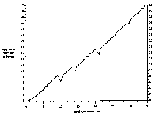
Figure 21.6 Sending
of 32768 bytes of data from slip
to vangogh.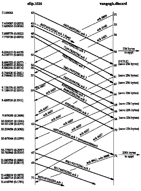
Figure 21.7 Packet
exchange for retransmission around the 10-second mark.21.6 Congestion Avoidance Algorithm
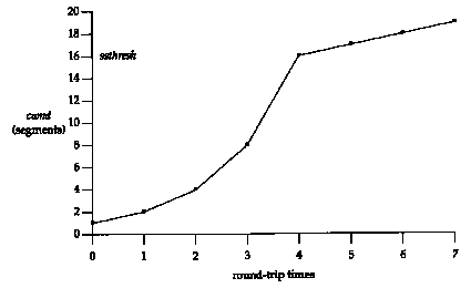
Figure 21.8 Visualization
of slow start and congestion avoidance.21.7 Fast Retransmit and Fast Recovery Algorithms
We'll see what happens to the two variables cwnd
and ssthresh in the calculations in the next section.
21.8 Congestion Example (Continued)
SYN
ACK
-
timeout
retransmit
-
256
-
512
-
2
3
4
5
6
7
8
9
10
11
12
257:513(256)
513:769(256)
769:1025(256)
1025:1281(256)
1281:1537(256)
1537:1793(256)
-
ACK 257
ACK 513
ACK 769
ACK 1025
ACK 1281
slow start
cong. avoid
cong. avoid
cong. avoid
512
768
885
991
1089
512
512
512
512
512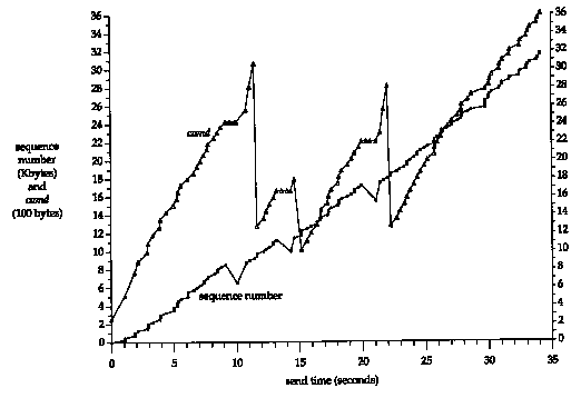
Figure 21.10 Value of cwnd and send sequence
number while data is being transmitted.
59
60
61
62
63
64
65
66
67
68
69
70
71
72
6657:6913(256)
8961:9217(256)
9217:9473(256)
9473:9729(256)
.
ACK 6657
ACK 6657
ACK 6657
ACK 6657
ACK 6657
ACK 6657
ACK 6657
ACK 6657
ACK 8961
duplicate ACK #1
duplicate ACK #2
duplicate ACK #3
retransmission
duplicate ACK #4
duplicate ACK #5
duplicate ACK #6
duplicate ACK #7
duplicate ACK #8
ACK of new data
2426
2426
1792
2048
2304
2560
2816
3072
1280
512
512
1024
1024
1024
1024
1024
1024
102421.9 Per-Route Metrics
21.10 ICMP Errors
An Example
slip % sock aix echo
run our sock program
test line
type this line
test line and it's echoed
SLIP link is brought down here
another line
then type this line and watch retransmissions
SLIP link is reestablished here
another line and the line and its echo are exchanged
line number 3
line number 3
the last line
SLIP link is brought down here, and not reestablished
read error: No route to host TCP finally gives up
1 0.0
slip.1035 > aix. echo: P 1:11(10) ack 1
2 0.212271 ( 0.2123)
aix.echo > slip.1035: P 1:11(10) ack 11
3 0.310685 ( 0.0984)
slip.1035 > aix.echo: . ack 11
SLIP link brought down here
4 174.758100 (174.4474)
slip.1035 > aix.echo: P 11:24(13) ack 11
5 174.759017 ( 0.0009)
sun > slip: icmp: host aix unreachable
6 177.150439 ( 2.3914)
slip.1035 > aix.echo: P 11:24(13) ack 11
7 177.151271 ( 0.0008)
sun > slip: icmp: host aix unreachable
8 182.150200 ( 4.9989)
slip.1035 > aix.echo: P 11:24(13) ack 11
9 182.151189 ( 0.0010)
sun > slip: icmp: host aix unreachable
10 192.149671 ( 9.9985)
slip.1035 > aix.echo: P 11:24(13) ack 11
11 192.150608 ( 0.0009)
sun > slip: icmp: host aix unreachable
12 212.148783 ( 19.9982)
slip.1035 > aix.echo: P 11:24(13) ack 11
13 212.149786 ( 0.0010)
sun > slip: icmp: host aix unreachable
SLIP link brought up here
14 252.146774 ( 39.9970)
slip.1035 > aix.echo: P 11:24(13) ack 11
15 252.439257 ( 0.2925)
aix.echo > slip.1035: P 11:24(13) ack 24
16 252.505331 ( 0.0661)
slip.1035 > aix.echo: . ack 24
17 261.977246 ( 9.4719)
slip.1035 > aix.echo: P 24:38(14) ack 24
18 262.158758 ( 0.1815)
aix.echo > slip.1035: P 24:38(14) ack 38
19 262.305086 ( 0.1463)
slip.1035 > aix.echo: . ack 38
SLIP link brought down here
20 458.155330 (195.8502)
slip.1035 > aix.echo: P 38:52(14) ack 38
21 458.156163 ( 0.0008)
sun > slip: icmp: host aix unreachable
22 461.136904 (2.9807)
slip.1035 > aix.echo: P 38:52(14) ack 38
23 461.137826 (0.0009)
sun > slip: icmp: host aix unreachable
24 467.136461 (5.9986)
slip.1035 > aix.echo: P 38:52(14) ack 38
25 467.137385 (0.0009)
sun > slip: icmp: host aix unreachable
26 479.135811 ( 11.9984)
slip.1035 > aix.echo: P 38:52(14) ack 38
27 479.136647 ( 0.0008)
sun > slip: icmp: host aix unreachable
28 503.134816 ( 23.9982)
slip.1035 > aix.echo: P 38:52(14) ack 38
29 503.135740 ( 0.0009)
sun > slip: icmp: host aix unreachabie
14 lines of output deleted here
44 1000.219573 ( 64.0959)
slip.1035 > aix.echo: P 38:52(14) ack 38
45 1000.220503 ( 0.0009)
sun > slip: icmp: host aix unreachable
46 1064.201281 ( 63.9808)
slip.1035 > aix.echo: R 52:52(0) ack 38
47 1064.202182 ( 0.0009)
sun > slip: icmp: host aix unreachable
21.11 Repacketization
bsdi % sock svr4 discard
hello there
first line gets sent OK
then we disconnect the Ethernet cable
line number 2
this line gets retransmitted
and 3
type this line before second line sent OK
then reconnect Ethernet cable
1 0.0
bsdi. 1032 > svr4.discard: P 1:13(12) ack 1
2 0.140489 ( 0.1405)
svr4.discard > bsdi.1032: . ack 13
Ethernet cable disconnected here
3 26.407696 (26.2672)
bsdi.1032 > svr4.discard: P 13:27(14) ack 1
4 27.639390 ( 1.2317)
bsdi.1032 > svr4.discard: P 13:27(14) ack 1
5 30.639453 ( 3.0001)
bsdi.1032 > svr4.discard: P 13:27(14) ack 1
third line typed here
6 36.639653 ( 6.0002)
bsdi.1032 > svr4.discard: P 13:33(20) ack 1
7 48.640131 (12.0005)
bsdi.1032 > svr4.discard: P 13:33(20) ack 1
8 72.640768 (24.0006)
bsdi.1032 > svr4.discard: P 13:33(20) ack 1
Ethernet cable reconnected here
9 72.719091 ( 0.0783)
svr4.discard > bsdi.1032: . ack 33
21.12 Summary
Exercises